I have always been surprised by the contrast between the grace of the main concept of binary search trees and implementation complexity of balanced Binary Search Trees (Red-Black Trees, AVL Trees and Treaps). I have recently looked through the “Algorithms” by Robert Sedgewick [1] and found a description of randomized search trees (I’ve also found the original [2]). It is just one third of a page long (nodes insertion, and one more page for deletion). There’s also a nice implementation of the operation on deleting nodes from a search tree. Here we'll talk about randomized search trees, their implementation in C++ and also results of a small author’s research as for these trees balance.
Let’s Go Step by Step
Since I am going to describe a complete implementation of a tree, we’ll have to start from the very beginning (professionals can skip several paragraphs). Each node of a binary tree will contain key key that manages all the processes, and a pair of pointers: left and right to the left and the right subtrees. If any pointer is NULL, the corresponding tree is empty, i.e. it’s simply missing. Besides, we are also going to need one more size field that will store the size of the tree with the root in the given node. We will represent the nodes with the help of the following structures:
struct node // a structure for the tree nodes representation
{
    int key;
    int size;
    node* left;
    node* right;
    node(int k) { key = k; left = right = 0; size = 1; }
};
The major feature of a binary tree is that any key is less than the root key in the left subtree and more than the root key in the right subtree. For clarity, we will consider that all keys are different. This feature (it’s shown in the picture on the right) allows us to organize the given key search easily, moving from the root either to the right, or to the left depending on the root key value. A recursive variant of the search function (we will review them only) looks like the following:
node* find(node* p, int k) // k key search in p tree
{
    if( !p ) return 0; // there’s no need to search in the empty tree
    if( k == p->key )
        return p;
    if( k < p->key )
        return find(p->left,k);
    else
        return find(p->right,k);
}
Let’s move on to inserting new keys in the tree. In the classic case, insertion repeats the search with one difference: when facing an empty pointer, we create a new node and «hook» it to the place, in which the dead end has been found. At first, I did not want to describe this function, as in the randomized case it operates a bit differently, but then I changed my mind. Anyway, let’s take a look at the following things:
node* insert(node* p, int k) // a classic insertion of a new node with k key in p tree
{
    if( !p ) return new node(k);
    if( p->key>k )
        p->left = insert(p->left,k);
    else
        p->right = insert(p->right,k);
    fixsize(p);
    return p;
}
First of all, any function modifying the given tree, returns the pointer to a new root (it does not matter, if it changed or not). Then the called function decides where to hook the tree. Secondly, since we have to store the tree size, when changing any of the subtrees, we should update the tree size itself. The following functions will be in charge of it:
int getsize(node* p) // a wrapper for size field. It operates with empty trees (t=NULL)
{
    if( !p ) return 0;
    return p->size;
}
void fixsize(node* p) //setting up a proper size of the tree
{
    p->size = getsize(p->left)+getsize(p->right)+1;
}
So what's wrong with the insert function? The thing is that this function does not guarantee the balance of the resulting tree. For example, if the keys are supplied in ascending order, the tree will result in a singly linked list (see the picture) with all related facilities. The major one is linear execution time of all operations on such tree. Meanwhile, this time is logarithmic for balanced trees. There are different ways to avoid imbalance. We can divide them into two classes: those guarantying balance (red-black trees, AVL trees) and those providing it in probability sense (treaps). In this case, probability to get an imbalance tree is negligible when a tree is big. I guess it’s no surprise that randomized trees belong to the second class.
Inserting in a Tree Root
Application of a special insertion of a new key is the essential component of randomization. As a result of insertion, the new key is in the tree root. This information is useful in many ways, as the access to recently added keys is really fast, hello to self-organizing lists. To carry out the insertion in the root, we are going to need the rotate function that performs a local transformation of the tree.

Do not forget to update the size of subtrees and return a new tree root.
node* rotateright(node* p) // right rotation round p node
{
    node* q = p->left;
    if( !q ) return p;
    p->left = q->right;
    q->right = p;
    q->size = p->size;
    fixsize(p);
    return q;
}
node* rotateleft(node* q) // left rotation round q node
{
node* p = q->right;
if( !p ) return q;
q->right = p->left;
p->left = q;
p->size = q->size;
fixsize(q);
return p;
}Now, let’s perform the insertion in the root. First of all, insert recursively a new key in the root of the left or the right subtrees (depending on the result of comparing with the root key) and perform a right (left) rotation that raises the necessary node to the tree root.
node* insertroot(node* p, int k) // inserting a new node with k key in p tree
{
    if( !p ) return new node(k);
    if( kkey )
    {
        p->left = insertroot(p->left,k);
        return rotateright(p);
    }
    else
    {
        p->right = insertroot(p->right,k);
        return rotateleft(p);
    }
} 
Randomized Insertion
We have finally made it to randomization. At the moment, we have two insertion functions – a simple one and the one in the root. Let’s make a randomized insertion from them. It is known that if we mix all the keys beforehand and build a tree from them (the keys are inserted according to a standard scheme in order that has been achieved after hashing), the built tree will be quite balanced (its height will be around 2log2n compared to log2n for a perfectly balanced tree). Please note, that in this case any of source keys can be a root. But what should we do, if we do not know beforehand, what keys we will have (for instance, they’re introduced into system during a tree usage). But all of that is actually simple. Since any key (including the one we will insert in the tree now) can be a root with 1/(n+1) probability (n is the tree size before insertion), we execute the insertion with the given probability and a recursive insertion in the right or the left subtree (depending on the key value in the root) with 1-1/(n+1) probability.
node* insert(node* p, int k) // a randomized insertion of a new node with k key in p tree
{
    if( !p ) return new node(k);
    if( rand()%(p->size+1)==0 )
        return insertroot(p,k);
    if( p->key>k )
        p->left = insert(p->left,k);
    else
        p->right = insert(p->right,k);
    fixsize(p);
    return p;
}
That’s it! Let’s check, how all of that works. Below is the example of building a tree from 500 nodes (keys from 0 to 499 came to the input in ascending order):

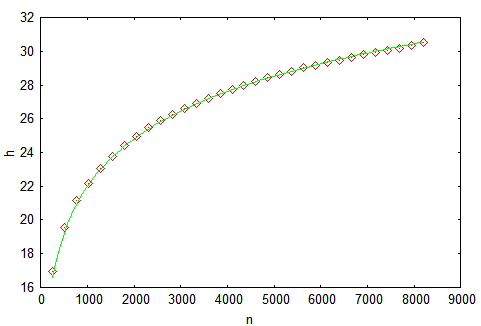
It’s not perfect, but it’s obviously not high. Let’s complicate the task. We will build a tree providing keys from 0 to 2^14-1 to the input (the prefect height is 14) and measure the height when building.
For reliability, let’s make a thousand of runs and average the result. We’ll get the following chart that shows results. Our results are highlighted with the marker, while the theoretical estimate from [3] is highlighted with the full line: h=4.3ln(n)-1.9ln(ln(n))-4. The main thing we can understand from the chart is that the probability theory is a great thing!
You should realize that the given chart reflects the average value of the tree height according to a great number of calculations. But how much can height differ in one specific calculation? The mentioned above article has a reply to this question as well. But we will just build a bar chart of heights distribution after the insertion of 4095 nodes.
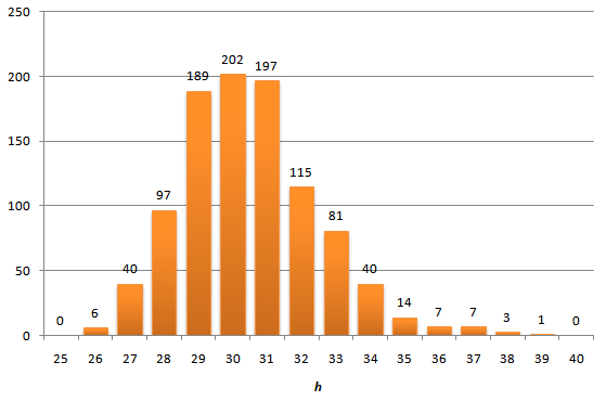
Anyway, there’s no crime. Distribution tails are short – the maximum height is 39, which does not exceed the average value.
Key Deletion
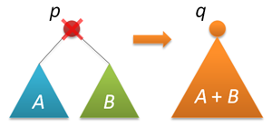
So, we have an imbalanced (at least in some way) tree. As for now, it does not support key deletion. That’s exactly what we are going to solve now. The described in manuals variant operates fast, but does not really look nice (in contrast to insertion). We will follow a different path. Before deleting nodes, we will learn how to join trees together. Let there be given two trees with p and q roots. Any key of the first tree is less than any key of the second tree. It is required to join these two trees into a single one. We can accept any of two roots as the root of a new tree, let it be p. In this case, we can leave the left p subtree as it is and fix the join of two trees to p on the right – the right p subtree and the whole q tree (they meet all the requirements).
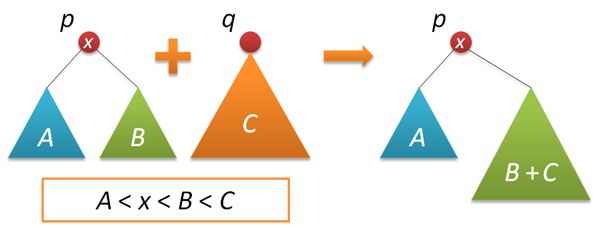
On the other hand, we can just as well make q node the root of a new tree. In the randomized implementation, we choose between these two alternatives in a random manner. Assume that the size of the left tree is n, while the right tree size is m. Then p is chosen to be a new root with n/(n+m) and q is chosen with m/(n+m) probability.
node* join(node* p, node* q) // joining two trees
{
    if( !p ) return q;
    if( !q ) return p;
    if( rand()%(p->size+q->size) < p->size )
    {
        p->right = join(p->right,q);
        fixsize(p);
        return p;
    }
    else
    {
        q->left = join(p,q->left);
        fixsize(q);
        return q;
    }
}
Now everything is ready for deletion. We are going to delete by the key. Look for the node with the specified key (reminding you that all keys are different) and delete this node from the tree. The search stage is the same as searching. Then we join the right and the left subtrees of the found node, delete the node and return the root of the joined tree.
node* remove(node* p, int k) // deleting from p tree the first found node with k key
{
    if( !p ) return p;
    if( p->key==k )
    {
        node* q = join(p->left,p->right);
        delete p;
        return q;
    }
    else if( kkey )
        p->left = remove(p->left,k);
    else
        p->right = remove(p->right,k);
    return p;
}
Let’s check that deletion does not affect balance of the tree. Build a tree with 215 keys, then delete half of them (with values from 0 to 214-1) and look at heights distribution.

There’s almost no difference, which was to be proved…
Instead of the Summary
Implementation simplicity and beauty are the doubtless advantages of Binary Search Trees. But what’s the drawback? What do we pay for it? First of all, the additional memory for storing subtrees sizes. One integer-valued field per each node. As for Red-Black Trees, we can do without additional fields. On the other hand, the tree size information is not useless, since it allows to organize the access to the data by number (sampling or order statistics search), which transforms our tree into an ordered array with feasible insertion and deletion of any elements. Secondly, though the operation time is logarithmic, the proportionality coefficient will not be small as all the operations are performed in two passes (up and down). Besides, insertion and deletion require random numbers. But there’s also the good news. At the search stage everything should operate really fast. Finally, logarithmic time is not guaranteed. There’s always a chance that a tree will be ill-balanced. But when there are ten thousand of nodes, such possibility is so negligible that it’s worth risking.
Thank you for your attention!
References
- “Algorithms in C++”, Robert Sedgewick
- Martinez, Conrado; Roura, Salvador (1998), Randomized binary search trees, Journal of the ACM (ACM Press)
- Reed, Bruce (2003), The height of a random binary search tree, Journal of the ACM 50 (3)
2 comments
Upload image