With this article I would like to continue the series of publications about the model of quantum computing. In the previous article I gave a brief introduction about reversibility of computing processes.
Dear reader, today I invite you to take a look at one of the simplest quantum algorithms, which shows the increase of efficiency in comparison with classical computing model. I am talking about Deutsch’s algorithm. We are also going to use Haskell to illustrate the approach and the Deutsch’s algorithm itself.
We will cover the fundamentals of the model of quantum computing and compare the classical and the quantum implementations of Deutsch’s algorithm. Also, you will finally understand the essence of quantum computations. So if someone is interested in this issue — you're welcome to join the journey.
Some History and a bit of Theory
In 1985, David Deutsch developed one of the first quantum algorithms. It was later known as the “basis” algorithm within the limits of the model of quantum computing. Deutsch’s algorithm shows a twofold efficiency increase in comparison to the classical computations when executing a program to solve a sort of a strange task. However, despite the low degree of the task applicability, the algorithm is significant. That’s why it is seen and mentioned in almost all the books related to quantum computations.
Suppose there is a function f, which has 1-bit inputs/outputs. The maximum number of such functions is four:
| № | Function | Indication | Type | Definition in Haskell |
|---|---|---|---|---|
| 1 |
f1(0) = 0 f1(1) = 0 |
0 | Constant |
|
| 2 |
f2(0) = 1 f2(1) = 1 |
1 | Constant |
|
| 3 |
f3(0) = 0 f3(1) = 1 |
id | Balanced |
|
| 4 |
f4(0) = 1 f4(1) = 0 |
not | Balanced |
|
The goal was to determine whether the function passed to an algorithm's input is constant or balanced. How can we do that? In the classical model of computations, we should call function f twice, then compare the results. If they are found to be equal, the function is constant, and if not, then balanced. One can hardly manage to solve this problem with a single function call. The following table illustrates the constant ambiguity in determining the type of the function, if one tries to determine its type with one call only:
| 0 | 1 | |
| 0 | f1 | f3 | f2 | f4 |
| 1 | f1 | f4 | f2 | f3 |
The fist column contains input values and the first row contains output values. The cells contain the functions returning some value at some argument. That is, functions f1 and f3 return 0 if the input value is 0. Since each cell of the table has two functions, it's impossible to solve the Deutsch's problem in one call in classical model of computations.
The model of quantum computing is another story. Here you can determine the type of a given function with a single call only. It happens due to the so-called quantum parallelism, when the function is called simultaneously at all possible values of its input parameters.
Since the model of quantum computing uses not bits, but qubits that can be located in an arbitrary linear superposition of quantum states, function f should be of another form here, in comparison to the classical model. It should be transformed into the so-called quantum oracle. It’s a unitary transformation (a certain type matrix) that operates on the input qubits the same way as the initial function f.
Simply put, the model of quantum computing represents a consequent multiplication of matrices by vectors, in which vectors represent qubits and matrices — unitary transformations. Quantum algorithms are usually described by means of circuits in which qubits are denoted by horizontal lines that are leading to and from boxes, that represent unitary transformations (gates). The box is labeled with designation of a unitary transformation. We can also use a special “measurement” operation. It transforms a qubit into a classical bit. This operation is denoted by a measuring device icon.
The quantum circuit of Deutsch’s algorithm looks the following way:

What can we see here? Two qubits are used in the algorithm. One of them is the basic one, the other one is auxiliary. Both of them are in the initial state. First of all, the auxiliary qubit is affected by X gate, which is the quantum analogue of operation NOT. After the action of the auxiliary qubit gate goes into |1> state. Then both qubits are simultaneously affected by the action of Hadamard gate H. It transforms the qubits from the basis quantum states into the equally probable superpositions and backwards. It turns the qubits 45 degrees in the two-dimensional Hilbert space. It’s time to call function f that is transformed into the quantum oracle. After the call (the only one), the first qubit if affected by the action of the Hadamard gate (we do not need the second one, as it has been auxiliary). Then it changes. There are two possibilities. If the value after the measurement is 0, the function is constant. If the value is 1, it is balanced.
All of this is a bit strange that it can seem magical. But really there’s nothing magical or strange about it at all. It’s all about quantum parallelism and transformation of the function into the quantum oracle. All the magic is hidden here and we are going to review why that happens so.
The Classic Version
To understand the main point here, we should review the classic implementation of the Deutsch’s algorithm. As we have illustrated above, to realize, whether the function is constant or balanced, we should call it twice. Let’s take a look at it in the code.
First of all, we will implement the functions. They will operate on a set of Integer integers. But not to deal with a great number of definitions and pattern matching (which would be the case when using either any Bool type, or some other defined type), we will use only two values of the set: 0 and 1. Thus, definitions of these functions are the following:
f1 :: Integer -> Integer
f1 _ = 0
f2 :: Integer -> Integer
f2 _ = 1
f3 ::
Integer -> Integer f3 = id
f4 :: Integer -> Integer
f4 x = (x + 1) `mod` 2It’s really simple to implement a function to solve Deutsch’s problem. Let's make it so that it prints the results of the measurements as a string:
deutsch :: (Integer -> Integer) -> IO ()
deutsch f = putStrLn (if f 0 == f 1
then "The function is constant."
else "The function is balanced.")As it has been promised, there are two calls for the given function. Well, to complete the implementation we can write a special function to test the already defined functions:
testDeutsch :: IO ()
testDeutsch = mapM_ deutsch [f1, f2, f3, f4]If we run it, the interpreter will print the following output:
> testDeutsch
The function is constant.
The function is constant.
The function is balanced.
The function is balanced.Exactly what we wanted to achieve.
Preparation for Implementation
Before we implement the algorithm, it is necessary to define quite a large set of auxiliary entities that will come in handy. First of all, we need two synonyms of types that will describe vectors and matrices. A special library with definitions of all the necessary things for linear algebra would be helpful. But what we want now is to implement the algorithm quickly and show how it looks in Haskell.
So, the two synonyms are the following:
type Vector a = [a]
type Matrix a = [Vector a]As we can see, a vector is just a list of some values, while a matrix is a list of vectors. But there is one important thing. A developer should always ensure the correctness and conformance of dimension of the data that has been represented with the help of the two types. For example, the multiplication operation of a matrix by a vector will not be able to check dimensions and guarantee the result adequacy. Thus, the developer has a honorable duty to control the lengths of the lists.
So qubits will be represented in the form of vectors, and unitary transformations or gates — in the form of matrices. Vectors and matrices should be complex-valued. This means that we should use the Data.Complex module. But complex numbers look quite lengthy in Haskell. Therefore, it is reasonable to define several auxiliary functions for the construction of complex-valued vectors and matrices of those that contain whole numbers. Here are these two functions:
vectorToComplex :: Integral a => Vector a -> Vector (Complex Double)
vectorToComplex = map (\i -> fromIntegral i :+ 0.0)
matrixToComplex :: Integral a => Matrix a -> Matrix (Complex Double)
matrixToComplex = map vectorToComplex
As we can see, the first function transforms the vector with counting values into a complex vector. The second function does the same thing with matrices. We can use them the following way:
qubitZero :: Vector (Complex Double)
qubitZero = vectorToComplex [1, 0]
qubitOne :: Vector (Complex Double)
qubitOne = vectorToComplex [0, 1]
gateX :: Matrix (Complex Double)
gateX = matrixToComplex [[0, 1],
[1, 0]]|0> and |1> qubits are defined here, as well as X gate, which represents the quantum operation NOT. And this is how to define H gate that represents the Hadamard transformation:
gateH :: Matrix (Complex Double)
gateH = ((1/sqrt 2) :+ 0.0) <*> matrixToComplex [[1, 1],
[1, -1]]We are also going to need a function that will combine several qubits into one quantum register. At its core, this function implements the tensor product of the vectors that represent qubits. This function is a joy to right in Haskell:
entangle :: Num a => Vector a -> Vector a -> Vector a
entangle q1 q2 = [qs1 * qs2 | qs1 <- q1, qs2 <- q2]This function connects two qubits that have been passed to its input. For instance, if we provide |0> and |0> qubits, we will see |00> qubit at the output. It goes without saying that we face the vector data model here. Therefore, |0> qubit is represented as [1, 0], and |00> qubit as [1, 0, 0, 0]. Being a thoughtful reader, you will be able to check the other pairs of basis qubits yourself. You can also check the qubits in the superpositions of the basis quantum states.
Now, let’s define the set of operators to perform quantum computations. There will be operators to multiply a matrix by a vector, and some other important operators as well.
apply :: Num a => Matrix a -> Vector a -> Vector a
apply m v = map (sum . zipWith (*) v) m
(|>) :: Num a => Vector a -> Matrix a -> Vector a
(|>) = flip applyapply function applies the defined gate to the defined qubit. A new qubit, or vector, is the result of its operation. By definition, it’s just the multiplication of a matrix by a vector. As for (|>) operator, it is used for the record beauty only. It is the same apply function, but with arguments that have been swapped. The vector comes first, and the matrix is the second. Besides, it’s an infix operator. That’s why we can write the application of a gate to a qubit as “qubitZero |> gateX”, which is quite fitting to the circuit record of quantum algorithms.
(<*>) :: Num a => a -> Matrix a -> Matrix a
c <*> m = map (map (c *)) mThis operator is used to multiply a number by a matrix. As a result, we obtain a matrix, all elements of which are equal to the multiplication of elements of the initial matrix by a defined number. We have already observed the operator use when determining Hadamard gate. Finally, the last definition:
(<+>) :: Num a => Matrix a -> Matrix a -> Matrix a
m1 <+> m2 = concatMap collateRows $ groups n [c <*> m2 | c <- concat m1]
where
n = length $ head m1
groups :: Int -> [a] -> [[a]]
groups i s | null s = []
| otherwise = let (h, t) = splitAt i s
in h : groups i t
collateRows :: [Matrix a] -> Matrix a
collateRows = map concat . transposeThis is the most complex definition in a module. This operator performs a tensor product of two matrices and creates (n * p) x (m * q) matrix of n x m and p x q matrices. The elements of the result-matrix are calculated according to the rules of the tensor product for matrices. This operator is required when creating gates for two qubit gates of a one-qubit gates.
How to Implement the Quantum Algorithm
It’s time to implement the quantum oracles for the four functions that have been mentioned at the beginning of the article. In the model of quantum computing, an oracle is a gate of a special type, which performs the computation of the specified function. Since there are two input qubits, the gates of oracles will represent a 4x4 matrices. To create them, we have to do a bit of quantum circuitry.
We will need to design four gates that perform the following unitary transformation:
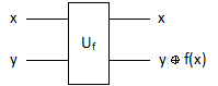
Let’s take a look at the first function. It is constant and returns 0 at any of its arguments. To build the gate, we should use the following table:
| x | y | f x | y + f x | Transformation |
|---|---|---|---|---|
| 0 | 0 | 0 | 0 | |00> -> |00> |
| 0 | 1 | 0 | 1 | |01> -> |01> |
| 1 | 0 | 0 | 0 | |10> -> |10> |
| 1 | 1 | 0 | 1 | |11> -> |11> |
To read the «Transformation» column, we should keep in mind that the qubit to the left of the arrow on the first position is the value of x, and the second — y. There’s also x value in the qubit on the right from the arrow on the first position. As for the second position, there is y + f x. It is clear that the unitary transformation is defined by a unitary 4 x 4 matrix.
Similarly, we can build the gate matrix for the second function. It is constant and always returns 1. Let’s make an auxiliary table that will help us to draw a unitary matrix represented by the gate. Here it is:
| x | y | f x | y + f x | Transformation |
|---|---|---|---|---|
| 0 | 0 | 0 | 0 | |00> -> |01> |
| 0 | 1 | 0 | 1 | |01> -> |00> |
| 1 | 0 | 0 | 0 | |10> -> |11> |
| 1 | 1 | 0 | 1 | |11> -> |10> |
In other words, the given unitary transformation should always apply the negation operation to the second qubit, with no regard of the first qubit value. The matrix of such transformation looks the following way:
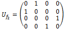
A cautious reader might have understood the way matrices for the third and the fourth functions look like. Anyway, building them is a nice exercise to understand all the mentioned things. Let’s take a look at the initial code to represent all the oracles:
f1' :: Matrix (Complex Double)
f1' = matrixToComplex [[1, 0, 0, 0],
[0, 1, 0, 0],
[0, 0, 1, 0],
[0, 0, 0, 1]]
f2' :: Matrix (Complex Double)
f2' = matrixToComplex [[0, 1, 0, 0],
[1, 0, 0, 0],
[0, 0, 0, 1],
[0, 0, 1, 0]]
f3' :: Matrix (Complex Double)
f3' = matrixToComplex [[1, 0, 0, 0],
[0, 1, 0, 0],
[0, 0, 0, 1],
[0, 0, 1, 0]]
f4' :: Matrix (Complex Double)
f4' = matrixToComplex [[0, 1, 0, 0],
[1, 0, 0, 0],
[0, 0, 1, 0],
[0, 0, 0, 1]]We have a little left to do. It’s time to implement the quantum version of the Deutsch’s algorithm, taking into account all the implemented auxiliary entities. Here’s the function:
deutsch' :: Matrix (Complex Double) -> IO ()
deutsch' f = do let (result:_) = measure circuit
case result of
'0' -> putStrLn "Function f is constant."
'1' -> putStrLn "Function f is balanced."
_ -> return ()
where
gateH2 = gateH <+> gateH
circuit = entangle qubitZero (qubitZero |> gateX) |> gateH2
|> f
|> gateH2
measure q = let result = map (\c -> round (realPart (c * conjugate c))) q
in case result of
[0, 1, 0, 0] -> "01"
[0, 0, 0, 1] -> "11"
_ -> "??"There is one thing about it. Locally defined function measure does not quite perform measurements that are taken in the framework of quantum computing. In the given case, this local function calculates the module of squares of amplitudes of all quantum states that enter the quantum register. Then, by means of comparing with two predefined lists, it returns a string describing the state of two qubits. The third sample of case expression is used for the code correctness only,
According to Deutsch’s algorithm, we are interested in the first qubit only. That’s why we compare it to 0 or 1 (again — the third sample is provided for the sake of correctness only). And if the measurement has returned 0, then the function is constant, and if 1, then balanced.
Now let's take a look at the local definition of circuit. It is the implementation of the quantum circuit of Deutsch’s algorithm. We have seen it twice in this article. As can be seen, with the help of the implemented operator (|>) quantum circuit is very nice shifted to the code in Haskell. What’s going on there? First of all, |0> (qubitZero) goes through gate X (gateX). Then, the result mixes with |0> qubit. As a result, there appears a new |01> register. After that, the quantum register goes through the double Hadamard gate, and then through oracle f, and through the double Hadamard gate again. As we can see, the quantum oracle, representing the study function, is used once only. It is the great peculiarity of Deutsch’s quantum algorithm
Finally, we will write a function to check the algorithm, just like we did it for the classic implementation. Actually, it’s pretty much the same. Here’s the code:
testDeutsch' :: IO ()
testDeutsch' = mapM_ deutsch' [f1', f2', f3', f4']Let's run it to see the result:
> testDeutsch’
Function f is constant.
Function f is constant.
Function f is balanced.
Function f is balanced.Summary
It might seem strange, but quantum version of the Deutsch’s algorithm is really better in contrast to the classic version. In order to determine the type of a function, it is really possible to run it only once. The thing is that we face parallelism within the limits of the model of quantum computing. It turns out that the function computes its values concurrently in all possible variants of values of its argument.
One might argue that the initial function was transformed to some matrix that had nothing in common with the initial variant and that that is the matrix running once. However, this argument is moot, as the unitary transformation obtained from the function is itself a function of one-to-one correspondence. Another thing is that we really should transform the function into a quantum oracle, but there’s nothing we can do about it.
By the way, we can implement Deutsch’s algorithm “in the hardware”. There are some physical processes. For example, passing photons or other similar particles that will help to implement the algorithm in a similar way.
Source code:
{-# OPTIONS_HADDOCK prune, ignore-exports #-}
{------------------------------------------------------------------------------}
{- | Deutsch’s Algorithm in Haskell.
Author: Roman V. Dushkin
-}
{------------------------------------------------------------------------------}
module Deutsch
(
-- * Classic implementation of Deutsch’s algorithm
deutsch,
testDeutsch,
-- * Qunatum implemenation of Deutsch’s algorithm
deutsch',
testDeutsch'
)
where
{-[ IMPORT SECTION ]-----------------------------------------------------------}
import Data.Complex
import Data.List (transpose)
{-[ SYNONYMS OF TYPES ]-----------------------------------------------------------}
-- | Synonym of a type to represent a vector. Simple list.
type Vector a = [a]
-- | Synonym of a type to represent a matrix. List of lists. By using this type
-- developer has to control the size of a list of lists and the size of each
-- individual list
type Matrix a = [Vector a]
{-[ FUNCTIONS ]------------------------------------------------------------------}
f1 :: Integer -> Integer
f1 _ = 0

f2 :: Integer -> Integer
f2 _ = 1

f3 :: Integer -> Integer
f3 = id

f4 :: Integer -> Integer
f4 x = (x + 1) `mod` 2
-- | Classic implementation of Deutsch’s algorithm.
deutsch :: (Integer -> Integer) -> IO ()
deutsch f = putStrLn (if f 0 == f 1
                        then "The function is constant."
                        else "The function is balanced.")
-- | Function to test classic implementation of Deutsch’s algorithm.
testDeutsch :: IO ()
testDeutsch = mapM_ deutsch [f1, f2, f3, f4]
vectorToComplex :: Integral a => Vector a -> Vector (Complex Double)
vectorToComplex = map (\i -> fromIntegral i :+ 0.0)

matrixToComplex :: Integral a => Matrix a -> Matrix (Complex Double)
matrixToComplex = map vectorToComplex
-- | Qubit |0>.
qubitZero :: Vector (Complex Double)
qubitZero = vectorToComplex [1, 0]
-- | Qubit |1>.
qubitOne :: Vector (Complex Double)
qubitOne = vectorToComplex [0, 1]
entangle :: Num a => Vector a -> Vector a -> Vector a
entangle q1 q2 = [qs1 * qs2 | qs1 <- q1, qs2 <- q2]
-- | Constant function, which returns a matrix representation of a quantum gate
-- X (NOT).
gateX :: Matrix (Complex Double)
gateX = matrixToComplex [[0, 1],
[1, 0]]
-- | Constant function, which returns a matrix representation of a quantum gate
-- H (Hadamard transform).
gateH :: Matrix (Complex Double)
gateH = ((1/sqrt 2) :+ 0.0) <*> matrixToComplex [[1,  1],
                                                 [1, -1]]
apply :: Num a => Matrix a -> Vector a -> Vector a
apply m v = map (sum . zipWith (*) v) m
(|>) :: Num a => Vector a -> Matrix a -> Vector a
(|>) = flip apply
(<*>) :: Num a => a -> Matrix a -> Matrix a
c <*> m = map (map (c *)) m
(<+>) :: Num a => Matrix a -> Matrix a -> Matrix a
m1 <+> m2 = concatMap collateRows $ groups n [c <*> m2 | c <- concat m1]
  where
    n = length $ head m1
    groups :: Int -> [a] -> [[a]]
    groups i s | null s = []
               | otherwise  = let (h, t) = splitAt i s
                              in   h : groups i t
    collateRows :: [Matrix a] -> Matrix a
    collateRows = map concat . transpose
-- | Function, which implements a quantum version of Deutsch’s algorithm
deutsch' :: Matrix (Complex Double) -> IO ()
deutsch' f = do let (result:_) = measure circuit
                case result of
                  '0' -> putStrLn "Function f is constant."
                  '1' -> putStrLn "Function f is balanced."
                  _   -> return ()
  where
    gateH2  = gateH <+> gateH
    circuit = entangle qubitZero (qubitZero |> gateX) |> gateH2
                                                      |> f
                                                      |> gateH2
    measure q = let result = map (\c -> round (realPart (c * conjugate c))) q
                in  case result of
                      [0, 1, 0, 0] -> "01"
                      [0, 0, 0, 1] -> "11"
                      _            -> "??"
-- | Function to test a quantum implementation of Deutsch’s algorithm.
testDeutsch' :: IO ()
testDeutsch' = mapM_ deutsch' [f1', f2', f3', f4']
-- | Unitary transformation to represent quantum oracle of a function
-- \f x = 0\.
f1' :: Matrix (Complex Double)
f1' = matrixToComplex [[1, 0, 0, 0],
[0, 1, 0, 0],
[0, 0, 1, 0],
[0, 0, 0, 1]]
-- | Unitary transformation to represent quantum oracle of a function
-- \f x = 1\.
f2' :: Matrix (Complex Double)
f2' = matrixToComplex [[0, 1, 0, 0],
[1, 0, 0, 0],
[0, 0, 0, 1],
[0, 0, 1, 0]]
-- | Unitary transformation to represent quantum oracle of a function
-- \f x = x\.
f3' :: Matrix (Complex Double)
f3' = matrixToComplex [[1, 0, 0, 0],
[0, 1, 0, 0],
[0, 0, 0, 1],
[0, 0, 1, 0]]
-- | Unitary transformation to represent quantum oracle of a function
-- \f x = not x\.
f4' :: Matrix (Complex Double)
f4' = matrixToComplex [[0, 1, 0, 0],
[1, 0, 0, 0],
[0, 0, 1, 0],
[0, 0, 0, 1]]
{-[ END OF MODULE ]-------------------------------------------------------------}
5 comments
There's a great one on hackage by Edward Kmett called linear :)
hackage.haskell.org/package/linear
Upload image