Deep Blue beat Kasparov at chess in 1997.
Watson beat the brightest trivia minds at Jeopardy in 2011.
Can you tell Fido from Mittens in 2013?
The picture and quote are taken from the challenge at Kaggle that took place in autumn last year.
Looking ahead, we can fairly enough reply “Yes” to the question. The ten leaders coped with the task by 98.8%, which can not but impress.
But where does such question come from? Why have classification tasks been (and still are) beyond programs’ capacity, though a four year old child can cope with them? Why is it more difficult to identify objects of the world than to play chess? What is deep learning and why are cats mentioned so often in related posts? Let’s talk about it.
What Does “Detect” Mean?
Suppose there are two categories and a great number of pictures to be apportioned to the two corresponding piles. According to what principle are we going to do that?
Nobody knows, actually, but a common approach is as follows: we will look for some “interesting” pieces of data that can be met in one of the categories only. Such data pieces are called features, and the approach itself is called feature detection. There are plenty of arguments for the fact that biological brain operates in a similar manner. The first of them is the famous experiment of Hubel & Wiesel on the cells of cat (again) visual cortex.
We never know beforehand, which parts of our picture can be used as good features. Anything can be associated with them: image parts, form, size or color. A feature itself can even be missing at the picture. But it can be expressed in a parameter that has been obtained from the initial data, for example, after the edge detection use. Okay, let’s take a look at some examples with increasing complication:
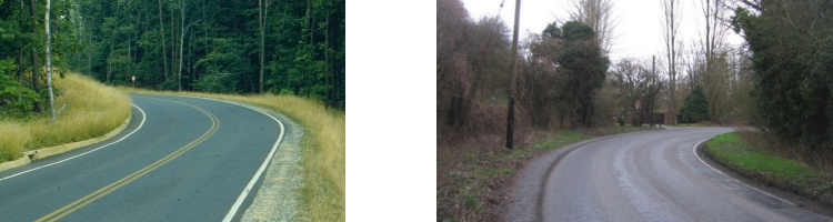
Let’s assume that we want to make a Google car that can distinguish right from the left turns and twist the steering wheel accordingly. We can compound the rule of identifying a good feature in simple words. Cut off the upper half of the picture and highlight the area of a definite shade (asphalt). Then apply some logarithmic curve to it on the left. If the whole asphalt is located under the curve, it’s the right turn, if otherwise – the left turn. We can have several curves in case of turns of different curvature, and, of course, a set of asphalt shades including dry and wet states. Our feature will be useless on dirt roads, though.
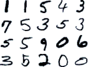
An example from the data set of hand-written MNIST numbers. I guess everyone being familiar with machine learning has seen this picture. Each number has typical geometric entities that define the kind of number it is – a squiggle at the bottom of two, an oblique stroke through the entire field of one, two joined circles of eight, etc. We can create a set of filters that will choose these significant elements, and then apply these filters by turns to our image. The one showing the best result is most likely the right answer.
These filters will look something like this:

It’s the picture from the course by Geoffrey Hinton “Neural networks for machine learning”. Pay attention to 7 and 9 numbers. They miss the lower part. The thing is that it’s the same for seven and nine and contains no useful information for identifying. Therefore, a neuronet that had chosen these features ignored the element. We usually use regular single-layer neuronetworks or something similar to get such feature filters.
Let’s stick to the point. What about this?
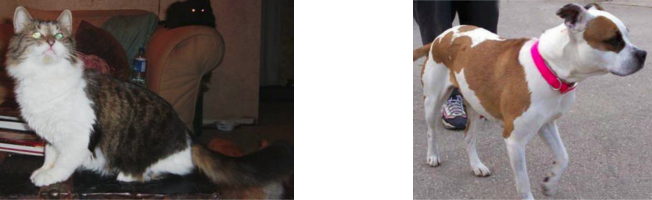
There are plenty of differences between these two pictures, such as brightness and color levels. White color prevails in the left part of the left picture. As for the right picture, white color prevails in its right part. But what we need to choose is the differences that will unambiguously detect cats or dogs. For example, the following two pictures can be identified as belonging to one category:
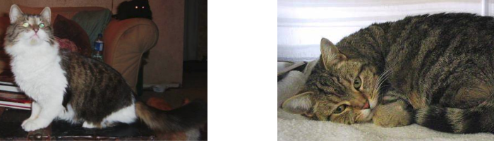
If we look at them for a long time and try to define things they have in common, the only thing coming to mind is the form of their ears. They are more or less the same but a bit bent on the right. But it’s also a coincidence. It’s easy to imagine (and find examples from the data set) a picture, in which the cat looks in a different direction, tilts the head, or it’s captured from the back. All other things differ. The scale, hair length and color, the pose, the background… They have nothing in common. However, a small device in your head can accurately assign these two pictures to one category. As for the upper two pictures, it will identify them as belonging to different categories. As for me, I cannot but admire the fact that such a powerful device is so close to us. Nevertheless, we can not comprehend the way it operates.
Five Minutes of Optimism (and Theory)
Okay. But what if we try and ask an innocent question? How do cats and dogs differ? We can easily begin this list: hair, fluffiness, the form of paws, characteristic poses. Or, for example, the fact that cats have no eyebrows. The problem is that all of these distinctive features are expressed in terms of pixels. We can not use them in an algorithm until we explain to it, what eyebrows are and where they should be located, or what paws are and where they grow from. Moreover, we execute all of detection algorithms in order to understand that it is a cat – a creature we can apply the notions of “whiskers”, “paws” and “tail” to. Without it, we can not even say with reasonable confidence, where the wallpapers or the sofa ends and the cat begins. We’ve come full circle.
And still, we can draw some conclusion from it. When formulating the features in the previous examples, we judged by possible object variability. The road turn can only be either left, or right and there are no other variants (besides going straight, but there’s nothing to do there anyway). Plus, the road building standards guarantee that the turn will be quite smooth, and not at a straight angle. Therefore, we build our feature in such a way so that it would accept various curvature of the turn, a specified set of hues of the road surface and that would be it for the possible variability. The next example: 1 number can be written in various handwritings and all variants will differ from each other. But it should not necessarily contain a straight (or an inclined) vertical line, otherwise it will be stop being one. When preparing the feature filter, we leave some space for the classifier variability.

If we look at the picture one more time, we will see that the active part of the filter for one represents a thick line that allows to draw a line with different tilts and a possible acute angle in the upper part.
In case with cats “the space for maneuver” for our objects becomes immeasurably huge. The cats in the picture can be of various breeds, big or small, against any background. They can be partially obscured by some object and they can definitely pose in thousands of different ways. We have not even mentioned rotation and cropping – the bane of all classifiers. It seems impossible to create a flat filter that similar to the previous one, and will be able to take all of these changes into account. Let’s imagine the combination of thousands of different poses in one picture. We will get a shapeless spot that will respond positively to everything. Thus, the sought features should represent a more complex structure. It’s not clear yet, what kind of structure it should be, but it should definitely have a feasibility to consider all these possible changes in it.
The “not clear yet” has lasted for quite a while, — during the bigger part of the deep learning history. Suddenly, people realized the following idea about the world. It sounds something like:
All things consist of other smaller and more elementary things.
Saying “all things”, I literally mean everything we are able to learn. Since this post is about the vision, I am talking about depicted outward objects. We can represent any visible object in the form of a composition of some stable elements. The latter consist of geometric figures being a combination of lines and angles located in a certain order. Something like the following:

(Since I haven’t found a good informative picture, I cut this one from Andre Ng (Coursera founder) speech about deep learning.
By, the way, within the limits of blue sky thinking, we could say that our speech and a natural language (that have been considered to be problems of the artificial intelligence for quite a while) represent a structural hierarchy, in which letters form words, and words form word-combinations that form sentences and texts. When coming across a new word, we do not have to learn its letters all over again. As for unknown texts, we do not consider them as something requiring specific memorizing and learning. Checking with the history, there are plenty of approaches (for the most part, they were more scientific) that have already stated it:
1. In 1959 the already mentioned Hubel and Wiesel discovered cells in the visual cortex that reacted to certain symbols on screen. They also discovered existence of other cells “at a higher level” that reacted to certain stable combination of signals from cells of the first level. In this basis, they supposed that there existed an entire hierarchy of similar cells-detectors.
A great video fragment of the experiment that demonstrates the way they discovered the necessary feature by chance. It made the neuron fire after they moved the sample a bit aside and a piece of glass slipped into the projector.
Warning: If you’re a sensitive person, you’d better not watch the video as they carry out the experiment on a cat.
2. Somewhere in 2000s there appeared the deep learning term with regard to neural networks that have not just one layer of neurons, but plenty of them. Thus, neuronetworks can be taught several feature levels. This architecture has strongly valid advantages. The more levels there are in a network, the more complex structures it can express. But there arises a problem of the way such networks can be taught. The backpropagation algorithm that was commonly used, can not operate well with a big number of layers. There appear several different models for these purposes: autoencoders, restricted Boltzmann machines, etc.
3. In 2004 Jeff Hawkins wrote in his “On Intelligence” book that the hierarchic approach is great and future belongs to it. He was a bit late, but I still want to mention him as he derived this thought in plain language from absolutely ordinary things. He is the person being far from machine learning and even used to say that neural networks were a bad idea. You should definitely read this book as it’s really inspiring.
Something about Codes
Thus, we have a hypothesis. Instead of stuffing the learning algorithm with 1024x768 pixels and watch it missing memory and being unable to understand what pixels are important to identify, we will extract some hierarchic structure from the picture. It will consist of different levels. The first one will contain some basic, structurally simple picture elements — its structural bricks: boundaries, strokes and segments. The higher level will contain stable feature combinations of the first level (for example, angles). The next level will contain features built from the previous ones (geometric figures, etc.). But where can we get such a structure for a single picture from?
Now, let’s talk about code.
To represent an object of the real world in the computer, we use some set of rules to convert this object piece by piece to the digital form. For example, one letter can be represented as an integer from ASCII table. As for the picture, it will be divided into plenty of small pixels. Each of them will be expressed with a set of numbers rendering brightness and color information. There are great many of color representing models. It does matter, which one of them we are going to use. But for simplicity, let’s imagine a black-and-white world, in which one pixel is represented with a number from 0 to 1 that will express its brightness – from black to white.
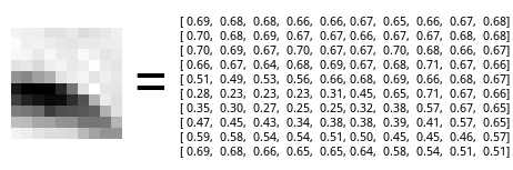
What’s wrong with this representing? Each pixel here is independent. It conveys just a small part of the information about the final picture. On the one hand, it is good when we need to save a picture somewhere or pass it through the network, as it occupies less space. On the other hand, it is uncomfortable for detection. In our case we can see an oblique stroke (with a bit of curve) in the lower part of the picture. It’s hard to tell, but it is a part of the nose contour from the picture of the face. In the given case, important pixels are the ones leaving this strike. The boundary between black and white is important. As for the subtle play of light in light-gray hues of the upper part of the square, it is not important at all. Thus, there’s no need to spend computing resources on it. This view requires dealing with all pixels at once. Each of them is not better than another one.
Now, let’s imagine another code. Separate this square into a linear sum of other squares. Each of them is multiplied by a coefficient. Let’s imagine a lot of dark glass plates with various transparency degrees. There are various strokes on each of the plates: vertical, horizontal, etc. Put the plates on top of each other and form a pile. Adjust transparency in a way to get something similar to our picture. It should not be perfect, but enough for identifying purposes.
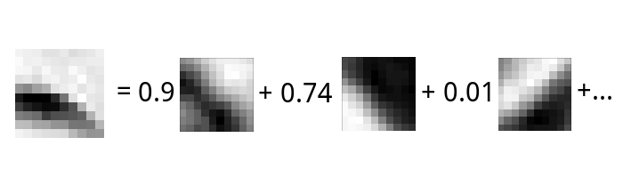
The new code consists of functional elements. Each of them says something about the presence of some separate component in the initial square. A component with a vertical stroke has 0.01 coefficient. So, we understand that there’s little “verticality” in the sample. But there’re plenty of oblique strokes in this component (see the first coefficient). If we select components of the new code, its dictionary, in an independent way, we can expect that there will be few non-zero coefficients. Such a code is called sparse.
We can see useful features of such representation by the example of one of applications named denoising autoencoder. If we divide this picture into small squares of 10x10 size and select appropriate code, we will be able to perform this image denoising with impressive efficiency and convert the noised image to code and restore it (here you will find an example). It shows that code is insensitive to random noise and saves those parts of the image being necessary for object identifying. That’s why we think that there became “less” noise after restoration.
On the other hand, it turns out that the new code is more heavyweight, depending on the number of components. For example, a square of 10x10 pixels can become much heavier.
There is evidence that the visual cortex encodes 14x14 pixels (of 196 size) with the help of around 100,000 neurons.
We have suddenly got hierarchy of the first level that consists of elements of the code dictionary. The elements represent strokes and boundaries. The only thing we have to get is the dictionary.
Five Minutes of Practice
Let’s use scikit-learn package — the library for machine learning for SciPy (Python). In particular, we will utilize MiniBatchDictionaryLearning class. We chose MiniBatch, as the algorithm will not be for the entire data set at once. It will be applied for small, randomly selected data packs. The process is quite simple and can be written in ten lines of code:
from sklearn.decomposition import MiniBatchDictionaryLearning
from sklearn.feature_extraction.image import extract_patches_2d
from sklearn import preprocessing
from scipy.misc import lena
lena = lena() / 256.0 # test image
data = extract_patches_2d(lena, (10, 10), max_patches=1000) # extract a thousand of 10x10 pieces – they are the teaching selection
data = preprocessing.scale(data.reshape(data.shape[0], -1)) # rescaling – move values symmetrically to null; the standard deviation should be equal to 1
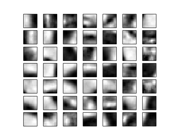
learning = MiniBatchDictionaryLearning(n_components=49)
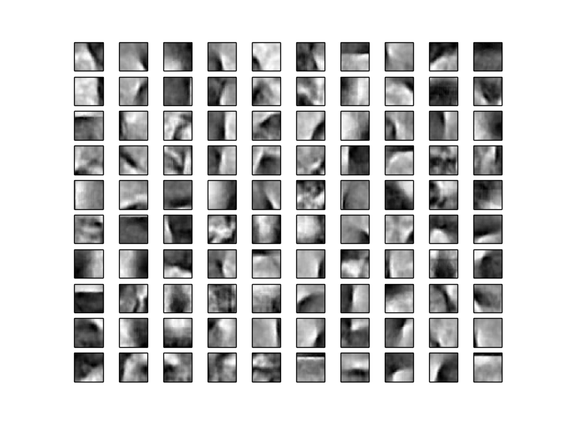
features = learning.fit(data).components_If we drew those parts being located in features, we would get something of the kind:
The output via pylab:
import pylab as pl
for i, feature in enumerate(features):
    pl.subplot(7, 7, i + 1)
    pl.imshow(feature.reshape(10, 10),
              cmap=pl.cm.gray_r, interpolation='nearest')
    pl.xticks(())
    pl.yticks(())
pl.show()
That’s where we can stop for a little while and recall why we have started all of this. We wanted to get a set of quite independent “structural bricks” forming the depicted object. In order to gain it, we have cut a great many of small square pieces and applied an algorithm. Then we noticed that it is possible to represent with adequate authenticity degree all of the small square pieces in the form of such elements. Since we face only edges and boundaries on the level of 10x10 pixels, we will get them as a result and all of them will be different.
We can use the encoded representation as a detector. To understand, whether the randomly chosen piece of the picture is an edge or a boundary, we ask scikit to choose the equivalent code. Like this:
patch = lena[0:10, 0:10]
code = learning.transform(patch)
If any of the code components has quite a big coefficient in contrast to other ones, we know that this signals about the presence of the appropriate vertical, horizontal or any other stroke. If all components are about the same, it means that a single-layer noise or a background is depicted here. And we know that it is of no interest.
But let’s move on. We are going to need a few more transformations.
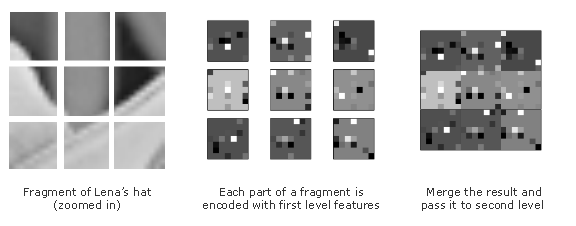
So, we can express any 10x10 fragment with the help of a chain consisting of 49 numbers. Each of them will denote the coefficient of transparency for the corresponding component of the picture above. Now, let’s write these 49 numbers in the form of a square 7x7 matrix and draw what we’ve got.
Here are two examples for clarity:
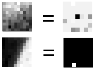
On the left is the fragment of the original image. On the right is its encoded representation, in which each pixel is the level of presence of the appropriate component (the lighter, the more). We can notice that the first (upper) fragment has no distinct stroke. It code looks like a merge of everything in a weak pale-gray intensity. The second fragment has one component only. All other are equal to null.
In order to improve the second hierarchy level, let’s take a bigger fragment of the picture (so that it could contain several small ones, say, 30x30). Now let’s cut it into small garments and represent each of them encoded. Then, join all of them and teach another DictionaryLearning on the basis of the data. The logic is simple: if the primary idea is right, the adjoined edges and boundaries should also form stable and repeating combinations.
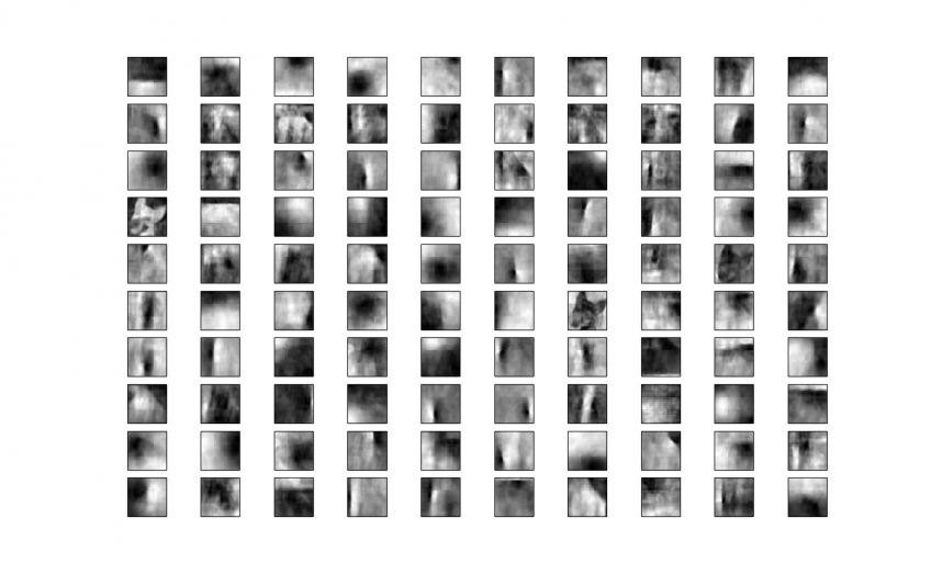
At first glance, it does not look like something meaningful, but it only seems so. That’s what we get at the second hierarchy level, which we practiced on people faces.
However, the size of a fragment here is bigger — 25x25 instead of 10x10. One of the unpleasant features of this approach is the need to adjust the size of the most "smallest unit of meaning".
There occur some difficulties with drawing the obtained “dictionary”, as the second level is taught on the first level code. Its components will look like a mixed hash of points from the picture above. That’s why we should take a step down and split these components into parts, then “decode” them with the help of the first level. We are not going to review this process in details.
Then we grow the levels on the same principle. For example, here’s the third level. We are going to see something interesting in it:
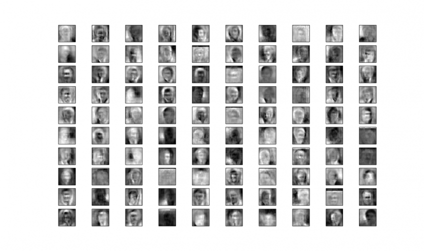
Each face here is a 160x160 feature. These are the most common viewings: frontal, half-turn, right and left, plus various skin colors. Each feature consists of two layers. First of all, they allow performing a quick check of test images for validity. Secondly, they provide additional “freedom”: contours and edges can deviate from perfect lines. But until they are within the limits of features of their level, they can signal upward about their presence.
Not bad, hah?
That’s it? We have won?
Obviously, we haven’t. If we run the script I draw all these sets with, we will see quite a dispiriting situation with the sought data set about cats and dogs. Level after level, it will return us the same features representing a bit curved boundaries.
We fetched one of dogs, but it is a pure coincidence — because similar silhouette met in the sample, for example, twice. If we run the script again, it may not appear.
Our approach suffers due to the same reason we criticized regular feed-forward neuron networks. During the process of learning, DictionaryLearning tries to find some common places and structural components of the chosen picture fragments. In case with faces, it turned out well as they are more or less alike: elongate oval forms with some number of deviations. As for several hierarchy levels, they provide more freedom in this regard. In case with cats, it did not turn out well as it was hard to find two alike silhouettes. The algorithm wouldn’t find anything common between the pictures in the test selection, excluding the first levels, in which we dealt with strokes and boundaries. Fail. It’s another dead end.
Ideas for Future
Actually, come to think of it, selection with a great number of different cats is good in a way that it covers varieties of breeds, poses, sizes and colors. But it may be not so successful for teaching our brain. After all, we teach by means of frequent repetitions and object study and not by looking through all possible variations. To learn playing piano, we should play scales all the time. It would be great if we would have to just listen to a thousand of classics.
Thus, the first idea is to step aside from variety in a selection and focus on one object in the same scene, but, say, in different positions.
The second idea follows the first one. It has already been mentioned by Jeff Hawkins and also by other people. We should try to benefit from time. After all, variety of forms and poses belonging to one object is temporal. To begin with, we can group successively coming pictures knowing that they depict one and the same cat that poses a bit differently in each of them. It means that we will have to change the teaching selection cardinally and use Youtube videos found by “kitty wakes up” query. We are going to talk about it in the following post.
You Can Look at the Code
… at github. Launch it with python train.py myimage.jpg (you can also specify the folder with pictures). There are also additional setting parameters: number of levels, size of fragments, etc. It requires scipy, scikit-learn and matplotlib.
Useful links
-
A Primer on Deep Learning. An informative post with the history of the problem, a short introduction and much more beautiful pictures.
-
UFLDL Tutorial. A tutorial by Andrew Ng from Stanford. To get your hands dirty. It contains literally everything you need to get familiar with the way all of it works. The introduction, the process mathematics, parallels with feed-forward networks, illustrated examples and exercises in Matlab/Octave
-
Neural Networks and Deep Learning. A free online book. Unfortunately, it’s not finished yet. It describes the basis in simple phrases, starting with perceptrons, neuron models, etc.
-
Geoffrey Hinton tells about new generations of neuron networks
-
The last talk with Hawkins, in which he covers briefly the ideas of his book, but more specifically. He tells about the things an intelligent algorithm should be able to do, about the fact that well-known features of a human brain tell us about it. He also dwells on neuron networks drawbacks and sparse coding advantages.
1 comment
In that particular paper circular patches represented with SIFT descriptors are used as 'codewords' and clustered to build a vocabulary/dictionary. Images are then represented using that vocabulary. The fact that the patches are circular rather than square makes them rotationally invariant. Furthermore, SIFT descriptors are one of the state-of-the-art methods of describing shape and are scale-invariant. This allows a more descriptive vocabulary to built.
At this stage, you basically have a set of images described by their most prominent shape features in the form of feature vectors. You can then use any algorithms to classify those. A good choice is SVM as it weighs the features based on how much they affect the decision boundary between classes. Thus, if you investigate your top support vectors, you could find not necessarily the common characteristics in a particular class, but rather, the characteristics that differentiate that class from all the other classes. I can see that the DictionaryLearning algorithms also tries to optimize the features used so that could be a good choice too.
This method could improve results in difficult cases where there is large intra-class variance, as you described. The complex descriptors would make the algorithm more robust and accurate in general.
Upload image