Building a Minimal Convex Hull

Convex Hull

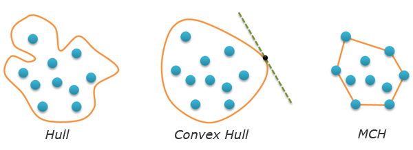
Since I have recently become interested in convex hulls, I decided to go on telling you about the algorithmic geometry. Today we are going to review the building of the so-called minimal convex hulls. Though the picture on the right provides an exhaustive explanation of what they actually are, you will find more formal definitions and two classical examples below.

Minimal Convex Hull Notion

Let the plane have a given finite number of A points. The hull of this set is any closed line H with no self-intersections, so that all A points are within this line. If H is convex (for example, any tangent to this line does not intersect it in any point), the corresponding hull is also named convex. Finally, a minimal convex hull is a convex hull of the minimal length (minimal perimeter). I have not checked (I guess it can be proved by contradiction), but it seems obvious that a minimal convex hull is required to be convex. All the mentioned definitions are depicted below:

Convex Hull, Minimal Convex Hull

The main peculiarity of a minimal convex hull of A points set is the fact that this hull represents a convex polygon. Its vertices are some points of A. Therefore, the task of minimal convex hull searching comes to selecting and ordering the necessary points. Ordering is necessary, as an output of an algorithm should be a polygon (i.e. a sequence of vertices). Let’s add an additional condition for the order of vertex location – the orientation of a polygon should be positive. Reminding you that positive is the counter clockwise traversing of a figure.

The task of building a minimal convex hull is considered to be one of the simplest tasks in computational geometry. There are plenty of different algorithms for it. We are going to review two of them: Graham scan and Jarvis march. Their description is illustrated by the code in Python. Both algorithms require orientation function which was reviewed in details in my previous post. Keep in mind that this function determines from which side C point is located relatively to AB vector. The returned positive value corresponds to the left side (the three points constitute a «left turn» or counter-clockwise orientation), the negative one – to the right side («right turn» or clockwise orientation).

def orientation(A,B,C):
  return (B[0]-A[0])*(C[1]-B[1])-(B[1]-A[1])*(C[0]-B[0])

Graham scan

This algorithm has three steps. At the first step we search for any point in A that enters the minimal convex hull for sure. It’s no brainer that such point will be, for example, the one with the least x-coordinate (the left-most one in A). We will move this point (we’ll name it starting point) to the beginning of the list and will work with the remaining points. For certain reasons, the initial array of A points will not be changed. We’re going to use the indirect addressing for all manipulations with the points. We’ll create P list that will store numbers of the points (their position in A array). Thus, at the first stage of the algorithm the first point in P should be the one with the least x-coordinate. The code:

def grahamscan(A):
  n = len(A) # number of points
  P = range(n) # number of point numbers 
  for i in range(1,n):
    if A[P[i]][0]


              The second step of Graham scan is sort a set of points in increasing order (except for P[0]) as for their left position with regard to the starting R=AP[0] point. We’ll say that B
              

              To achieve such ordering, we can apply any sort algorithm based on pair-wise comparison of these elements, for instance, a quicksort. Due to certain reasons, I will use the insertion sort.
              I will really appreciate if you can tell me how to apply the native Python sort here…
              Anyway, the insertion sort (do not forget about the indirect addressing and the fact that the starting point is not sorted):
              for i in range(2,n):
    j = i
    while j>1 and (rotate(A[P[0]],A[P[j-1]],A[P[j]])<0): 
      P[j], P[j-1] = P[j-1], P[j]
      j -= 1

              The following picture illustrates the sort result:
              
              If we now join the points in the obtained order, we will get a polygon that is not actually a convex.
              
              Let’s move on to the third step. All we have to do is to cut angles. In order to do that, we should traverse all the remaining vertices and delete the ones where the right turn happens (the angle in such vertex is bigger than straight). Create S stack (a list) and place the first two vertices into it (they enter the minimal convex hull for sure).
              S = [P[0],P[1]] Then look through all other vertices, keep track of recent three points, and find the angle formed by them. If orientation of these points is not counterclockwise, we can cut the angle by removing the last vertex from the stack. As soon as orientation is clockwise, it is no longer necessary to cut angles, so we will place the current vertex into the stack.
              for i in range(2,n):
    while orientation(A[S[-2]],A[S[-1]],A[P[i]])<0:
      del S[-1] # pop(S)
    S.append(P[i]) # push(S,P[i])

              As a result, the sought sequence of vertices is in S stack. It also has the needed orientation, which defines the minimal convex hull of A points set.
              return S 
              The time complexity of the first and the last steps of the algorithm is linear (or O(n)).
              Though the latter case has a nested loop, but each vertex inside this loop is pushed into the stack just once and can not be popped from there more than once. Therefore, the algorithm complexity is defined by the second step – sorting. That’s exactly why the insertion sort is not the best variant when n are big. If we replace it with the quicksort, we will get a summarized algorithm complexity O(nlogn).
              Can we improve this time? It is proved, that If the algorithm is based on the pair-wise comparison of points (like ours), the estimate can not be improved in the general case. From this point of view, Graham scan is the best solution here. Nevertheless, it has one characteristic which is not nice. It is not adaptive in the sense that it does not matter, how many vertices will enter the minimal convex hull (three, five, ten or n), the time will be linearly- logarithmic anyway. Jarvis march, which we are going to review below, has the mentioned adaptivity.
              Complete source code of the Graham Scan:
              def grahamscan(A):
  n = len(A) # number of points 
  P = range(n) # the list of point numbers 
  for i in range(1,n):
    if A[P[i]][0]1 and (rotate(A[P[0]],A[P[j-1]],A[P[j]])<0): 
      P[j], P[j-1] = P[j-1], P[j]
      j -= 1
  S = [P[0],P[1]] # create the stack
  for i in range(2,n):
    while rotate(A[S[-2]],A[S[-1]],A[P[i]])<0:
      del S[-1] # pop(S)
    S.append(P[i]) # push(S,P[i])
  return S

              Jarvis March
              Jarvis march (aka gift wrapping algorithm) is conceptually simpler than Graham Scan. There are two steps in it and it does not require sorting. The first step is the same – we need a starting point that enters the minimal convex hull for sure. Let’s take the left-most point from A:
              def jarvismarch(A):
  n = len(A)
  P = range(n)
  for i in range(1,n):
    if A[P[i]][0]

              At the second step we will build a minimal convex hull. The idea is that we make the starting vertex a current one, find the right-most point in A with regard to the current vertex and make it current, etc. The process finishes when the current vertex will again become the starting one. As soon as the point is inside the minimal convex hull, we can ignore it. That’s why we should create another H list that will store the minimal convex hull vertices in the correct order. Let’s place a starting vertex in it and move it to the end of P list (that’s exactly where we will find it and finish the algorithm).
              H = [P[0]]
  del P[0]
  P.append(H[0])

              Now let’s make an infinite loop. For each iteration loop find the left-most point of P with regard to the last vertex in H. If this vertex is the starting one, we will terminate the loop, otherwise – move the found vertex from P to H. After the loop is done, we will return H, which will contain the hull in it.
              while True:
    right = 0
    for i in range(1,len(P)):
      if rotate(A[H[-1]],A[P[right]],A[P[i]])<0:
        right = i
    if P[right]==H[0]: 
      break
    else:
      H.append(P[right])
      del P[right]
  return H

              Wow! I’ve managed to tell you about Jarvis march without using any pictures! The following one illustrates all of it!
              
              Let’s estimate time complexity of Jarvis march. The first step is linear (O(n)). The second one is more interesting. We have a nested loop, the number of external iterations that is equal to the number of h heights in the minimal convex hull. As for internal iterations, their quantity does not exceed n. So time complexity of the complete algorithm is O(hn). This formula is a bit unusual, as time complexity is defined not only by length of the input data, but also by the output length (output-sensitive algorithm). At worst, all points from A belong to the minimal convex hull (i.e. A is a convex polygon itself), then h=n and complexity becomes quadratic. At best (if all points from A are not on the same line), h=3 and complexity becomes linear. We just have to understand, which of the cases is ours. It is not a simple task, unless you we have a time machine. We can judge from the type of the task. If there are plenty of points and they evenly fill some area, Jarvis can be faster. But if the data is gathered at the boundary, Graham will be faster.
              **Time machine is quite a useful thing in the context of algorithms. Using it, we can immediately solve any task requiring a billion years of calculations. We should just start a program, get into the time machine, “fly” to the future and come back. We just have to find out the way of providing continuous computer operation for several billion years.
              The Complete code of Jarvis march:
              def jarvismarch(A):
  n = len(A)
  P = range(n)
  # start point
  for i in range(1,n):
    if A[P[i]][0]

              Summary
              To my mind, the task of building minimal convex hulls is quite a good way to begin with computational geometry. It is quite simple to think out an algorithm of your own, but it will certainly be a variation of Jarvis march. It has been affirmed that this task has plenty of applications, the bigger part of which is related to pattern recognition, clusterization, and so on. Besides that, this task is also used as a supplement for solving more difficult tasks of computational geometry. It is worth noting that this task has quite an interesting three-dimensional generalization.
              Thank you for reading the post!

Comments

Chao Xu 2:57PM on Friday, Dec 12, 2014

The definition of convex hull in this article is not the same as the standard terminology. I urge the author to use the standard terminologies(which is on the wikipedia page linked in the first paragraph.)

Kukuruku Hub 5:15PM on Friday, Dec 12, 2014

Hey Chao, thanks for pointing that out. We’ll try to edit it. Anything you would like to contribute?

Chao Xu 6:39PM on Friday, Dec 12, 2014
Here are some suggestions. I hope this produces the minimum amount of changes so the definition is equivalent to the standard terminology.
1. Instead of defining «hull», one can just state it as a «a closed curve that encloses all the points». «Hull» by itself isn’t used much outside this paragraph, and one can just say «closed curve» instead of «hull» to refer to the hull because there is little ambiguity.
2. One can then define what it means for a closed curve to be convex.
3. Replace all occurrence of «minimal convex hull» with «convex hull». Define the «convex hull of S» as the region bounded by the shortest convex closed curve that contains all the points in S.
4. Finally, one can state that what it means to «find the convex hull». State it as finding the boundary curve of the convex hull(which is the original «minimal convex hull»).
One can prove this definition is equivalent to the convex hull definition for finite set of points on the plane in wikipedia.
Kukuruku Hub 7:17PM on Friday, Dec 12, 2014

Thanks for a detailed feedback, Chao. We are looking into editing the article.

Off-topic: this conversation brought us to an interesting idea. What if we would let our users to edit articles and send diffs to authors, similar to git pull requests?

Wendell Smith 5:31PM on Friday, Dec 12, 2014

For sorting, I suggest using the

my_list.sort(key=keyfunc) syntax; see my comment on Reddit for more details.

Also, is the full code available somewhere (e.g. Github)? It would be nice to see! Thanks for the informative post!